MRI Physics: Spatial Localization

Jump to the sections on Frequency Encoding or Phase Encoding to see simulations of how those processes work.

Gradients

A magnetic resonance imaging sequence produces signal from all the tissue in the scanner (at least, all of the tissue within the transmit/receive coils). Without a means of spatial localization, all we would get is a single number for the entire body! Drs. Lauterbur and Mansfield discovered a way to separate signal from different parts of the body and received a Nobel prize for this accomplishment. In order to understand how they did it - and how MR scanners still work today - we need to understand magnetic gradients.

While the main magnetic field of the scanner (B₀) cannot change, we can add additional, smaller magnetic fields with changing electrical fields. As you may remember from physics, a changing electrical field produces a magnetic field; this is the basis of electromagnets. Each MR scanner has 3 sets of spatial encoding electrical coils to produce magnetic fields in the x, y, and z directions. These coils can be adjusted to produce not a constant field but a gradient, in other words a magnetic field that changes in strength depending on your position.

These magnetic fields are much weaker than B₀ and vary linearly across the x, y, or z direction. They can even be turned on in combinations to create a linear gradient in any arbitrary direction in space. By the Larmor equation, f = γ * B, so that if the magnetic field varies across space, the precession frequency of the protons will vary as well.

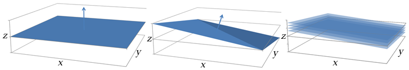
Illustration of how gradient coil combinations can give slices in an arbitrary axis. Left: A gradient along the z (vertical) axis gives a slice in the x-y plane. Center: A gradient formed by turning on all of the coils (x, y, and z) points towards the top-right corner of the patient. Right: Slices along this gradient are in an oblique plane.

Slice-Selection

Clearly, now that we have gradients, we can separate different parts of anatomy by frequency. We will start with the simplest type of separation: the imaging slice. Remember that protons only exchange energy efficiently if the frequency of the energy matches their precession frequency. Thus, the 90-degree and 180-degree pulses must be sent at the Larmor frequency of the proton. We can combine this with gradients to select a slice of the body to image:

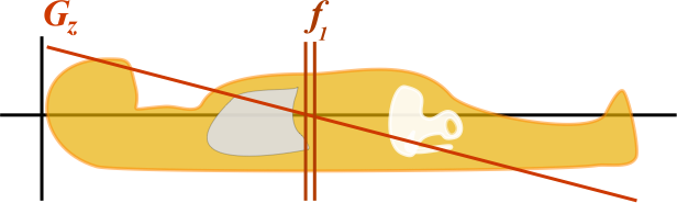
Illustration of a slice-select gradient in the z-axis. The gradient G_z gives increased magnetic field near the head and decreased magnetic field near the toes. At any point, by the Larmor equation, the frequency depends on the local magnetic field and thus on the z position ( f₁ = γ * B(z) ).

By turning on the magnetic field gradient, the protons at each position in the body experience a slightly different magnetic field - slightly more or less than B₀. Thus, we get a gradient of precession frequencies along the body that differ. By then altering the frequency of our 90-degree and 180-degree pulses, we will excite different protons. For this example, we will be using the slice-select gradient in the z-axis (along the axis of the body). Let's say that the adrenal glands lie at the center of the G_z gradient, so B = B₀ - and f = 63.9 MHz. The kidneys are a little below them so G_z is slightly less than 0, B = B₀ - 1%, and so f = 63.9 - 1% = 63.2 MHz. (In reality, magnetic field gradients are closer to the order of several hundredths of a percent over a couple centimeters, but I just used some easier numbers for the example.)

The scanner can select the particular slice to image by turning on the slice-select gradient and then altering the frequency of the excitation pulses (90, 180, and any inversion pulse) to match the frequency at the desired slice position. Protons not in the slice will not get excited since their Larmor frequency will not match the frequency of the pulse, thus they won't efficiently receive energy from the pulse. Note that the slice-select gradient doesn't have to be on during readout since no protons are being excited then - although the readout frequency will be centered at the particular frequency of that slice.

Fourier Transform

In order to understand how we determine spatial localization within a slice - frequency and phase encoding - we need to discuss the Fourier transform. Fourier (a French mathematician) realized that all signals, or oscillating functions, can be represented as a combination of simple sine and cosine waves. Each sine and cosine corresponds to a particular frequency in the signal. High frequencies correspond to rapidly changing features, while low frequencies (including zero, a constant signal) correspond to slowly changing features in the original signal. Fourier devised a method for transforming a signal in time, such as music, into the set of frequencies that compose it, and this is known as the Fourier transform.

While the intricacies of the Fourier transform are obviously much beyond the scope of this discussion, we will briefly discuss how it actually works. At the beginning, let us just discuss a signal composed of sine waves; we will get to the cosine part later. Sine waves have 2 important properties (actually, 3, but we'll get to that later): amplitude and frequency. As noted above, the frequency represents how fast the wave oscillates and the amplitude how high. A general sine wave can be written as an equation:

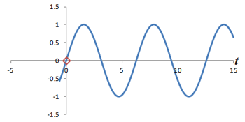
S(t) = A * sin(2 * π * f * t) for amplitude A and frequency f

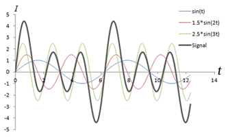
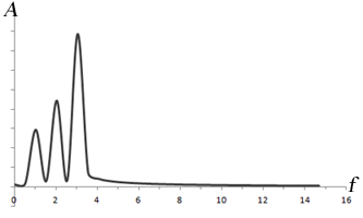
Left: Combination of 3 sine waves into an overall signal (dark gray), which has a more complex shape. Note that the different frequencies (sin(t), sin(2*t), sin(3*t)) have different signal strengths as well. Right: Fourier transform of the signal, which shows 3 peaks corresponding to the three signals. The heights of the peaks represent the strengths of each frequency component in the signal.

Mathematics of the Fourier Transform (Optional).

Phase. The Fourier transform provides a method for analyzing any arbitrary signal to obtain the amplitude (energy) of each frequency that is present in the signal by breaking it up into a combination of sine waves. Now, we have to discuss something a little more complicated than simple sine waves: phase. The most general way to describe a sine wave is actually:

sin(2 * π * f * t - φ)

φ represents the phase of the signal, which is how much it is shifted side-to-side; you can also think of it as a time delay.

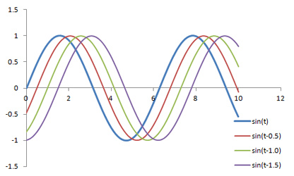
Graph of several sine waves with the same frequency and amplitudes but with varying phase shifts.

The simplified version of the Fourier transform we discussed above can't account for phase shifts - how does the Fourier transform actually do it? Well, instead of breaking the signal down simply into sine waves, we need to use both sines and cosines. Since cos(x) = sin(x + π/2) - in other words, the cosine is simply a phase-shifted version of the sine - it turns out that by using both sines and cosines we can take into account phase shifts as well.

Mathematics of Phase Shifts (optional).

We should note that, importantly, the Fourier transform cannot measure two phases at the same frequency. That is, if there are several sine waves in the signal with the same frequency but different phases, only one phase can be measured at that frequency. In other words, the Fourier transform is great at finding out how much (amplitude) of a given frequency is present, but it cannot decipher the combination of signal phases that may be present.

Sampling. There are a couple important practical things to know about the Fourier transform. Firstly, it is performed on data that is digitized by the MR hardware. This involves sampling or measuring the signal at a specific rate in time; the sampling rate determines the range of frequencies that can be measured by the Fourier transform, known as the Nyquist limit. Frequencies above this limit cause aliasing, which is the same phenomenon as seen in Phase-Contrast MRA and Doppler ultrasound. We cannot accurately measure frequencies that are above one half of the sampling rate. In other words, if the sampling rate - spacing of measurements in time - is ΔT, then we have to sample at twice the maximum frequency we want.

f_max = 1/2 * (1/ΔT), or 1/ΔT = 2 * f_max

What happens with any higher frequencies in the signal? The Fourier transform doesn't know what to do with them, so they get 'aliased' or wrapped to lower frequencies (i.e. within the range determined by the Nyquist limit). In the case of phase- or frequency-encoding, the signals associated with tissue at these locations are assigned to the wrong positions, causing overlapping structures. In the case of velocity measurements, often the velocity is mapped to a negative number.

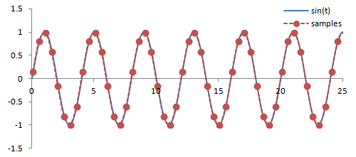
Illustration of sampling (red circles) and how this affects the inferred signal and frequency (red line). The blue line denotes the original signal. Sampling at or above twice the frequency of the signal leads to an accurate measurement of the frequency - one point for each peak/trough. Sampling below this frequency causes missed peaks/troughs and incorrect estimation of the signal's frequency.

Note that the Fourier transform of a digitized signal is referred to as the discrete-time Fourier transform. There are extremely fast computer algorithms for calculating the Fourier transform, known as fast Fourier transform or FFT. They work most efficiently on data with a length equal to a power of 2, which explains why our matrix sizes are often 128, 256, or 512.

Another important property of the Fourier transform is symmetry. It turns out that the Fourier transform (for any real signal, technically) actually gives two mirror-image halves. In the graph of the Fourier transform of the sine waves shown above, we just included one half, but the other half is exactly the same, just flipped along the vertical axis.

Frequency Encoding

Your browser does not support the HTML canvas. Frequency-Encoding Gradient: Off Low High

Your browser does not support the HTML canvas. Your browser does not support the HTML canvas.

Illustration of the frequency-encoding process. Left: Cartoon of four 'protons' in a slice of the abdomen with the rotating bars representing their precession. Top right: Plot of signal from each proton, over time. The colored lines correspond to the signals from each proton, and the gray line represents the total signal from the slice. Bottom right: Plot of the Fourier transform of the total signal, with peaks colored to represent the signals from each proton. Use the Play/Stop/Reset controls to start and stop the simulation; you can change the strength of the frequency-encoding gradient from Off to High.

The first within-slice localization technique we will discuss is frequency encoding. Frequency encoding is used to determine one axis in the xy-plane of the slice. Just like with slice selection, remember that the presence of a magnetic field gradient creates a corresponding gradient in the precession frequencies of the protons along that direction. Remember that we've already restricted the protons that are being excited to a particular slice by the slice-select gradient. Now, during readout we will turn on a gradient in the x-axis (for example). Thus, the frequencies of the protons in the slice will be slightly more or less than the slice average by the amount of this gradient. For example, the liver protons will precess slightly slower than the spleen protons.

The MR scanner will receive the entire signal from that slice (again, remember - only protons in that slice were excited). However, we have a tool to split up signals by frequency - the Fourier transform! Thus, we can split up the liver and spleen signals by performing a Fourier transform on the signal. The liver signal will be represented by the peaks at the low frequencies, and the spleen signal will be represented in the peaks at the high frequencies.

Mathematically, we can write this as follows. Let's denote the tissue intensity in a pixel in the liver as I_liver and that of a pixel in the spleen as I_spleen. Remember that with the gradient, the frequencies depend on the position of the pixels along the x-axis, so f_liver < f_spleen in our example with the gradient increasing left to right. Then

Signal = I_liver * sin(f_liver * t) + I_spleen * sin(f_spleen * t)

The Fourier transform of the Signal will give us a peak for every frequency, so we can find out the intensity at a point in the liver by calculating what frequency it corresponds to (i.e. how far are we along the x-axis and how strong is the gradient?), then looking up that frequency in the Fourier transform. As mentioned, this conversion depends on the gradient strength. Choice of gradient strength represents a trade-off between sampling time and signal-to-noise, a topic discussed in more detail in the separate section on bandwidth.

Mathematics of Frequency Encoding (optional).

The MR scanner acquires (listens to, samples) the signal over time. This is the sinusoidal oscillation just as you see in the simulation in this section or the drawing of sine waves earlier in this page. This signal is digitized and stored in the computer, in a matrix known as K-space. The Fourier transform of K-space is real space - the image.

Phase Encoding

Your browser does not support the HTML canvas. Frequency-Encoding Gradient: Off Low High Phase-Encoding Gradient: Off Low High

Your browser does not support the HTML canvas. Your browser does not support the HTML canvas.

Illustration of combined phase- and frequency-encoding. As with a real MR sequence, the phase encoding gradient is turned on and off first, then frequency encoding is applied. Left: Cartoon of four 'protons' in a slice of the abdomen with the rotating bars representing their precession. Top right: Plot of signal from each proton, over time. The colored lines correspond to the signals from each proton, and the gray line represents the total signal from the slice. Bottom right: Plot of the Fourier transform of the total signal, with peaks colored to represent the signals from each proton. Use the Play/Stop/Reset controls to start and stop the simulation; you can change the strength of the gradients from Off to High.

Thus far, we have discussed how to localize a proton to a slice and then along one axis within the slice. Both of these rely on changing the frequency of the protons. In order to localize along our third axis, we need to manipulate the phase of the protons. It turns out that this is pretty easy - all we have to do is turn on a gradient for a short amount of time, then turn it off. Once the gradient is off, the magnetic field strength B returns to its normal level (for the slice) - and so all of the protons go back to precessing at the exact same frequency. However, while the gradient was on, the protons were moving faster than their neighbors, so when the gradient is turned off they're still ahead - they have accumulated a phase shift.

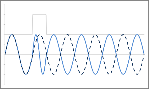
Example of a Phase Shift. The dashed blue line is the original precession plot. An RF gradient is applied (gray line), and the precession speeds up briefly (solid blue line). Note that even after the gradient is off, the two plots are out of sync.

So we can create phase shifts that vary across the y-axis, for example, by transiently turning on a gradient along that direction. In order to use both phase and frequency encoding, we first turn on the phase encoding gradient, then turn it off; this happens during the time we are waiting for the echo. At the time of the echo, we turn on the frequency-encoding gradient only. This changes the frequencies of the protons while we are measuring their precession - they still 'remember' their phase shifts from earlier.

Now, each pixel in the image has a unique frequency and phase combination. Unfortunately, as we alluded to earlier in the section on the Fourier transform, we cannot measure more than one phase per frequency. That means that we have no way of distinguishing signals along the phase-encoding direction. However, we can employ a trick - we can perform many different, separate phase-encoding gradients, measure the results from each of them, and then use the Fourier transform to figure out the phases. We need to repeat an entire MR sequence for each different phase-encoding gradient we need to measure, and we need to do one for each row of pixels in the image (i.e. if our image is 256 x 256, then we need to do 256 phase-encoding steps). Each phase-encoding step is stored as a different row in the K-space matrix.

What is the connection between multiple phase-encoding steps and the Fourier transform? Well, in fact, measuring successive phase shifts of a signal is equivalent to taking successive measurements of the same signal over time.

Left: Successive measurements of a sine wave over time. Right: Successive measurements of a sine wave at the same time but with different phase. Note how the measurements are actually the same.

In other words, phase shifts are similar to time shifts - and the rate at which the shifts are occurring represents a frequency that can be identified by the Fourier transform. Thus, if we use the traditional Fourier transform to analyze the signal in time, we obtain the frequencies in the signal, which we can use to decode amplitudes along the frequency-encoding axis. But if we use the Fourier transform to analyze the data 'on its head' along the phase encoding steps (for a single timepoint), we can obtain the phases in the signal, which we can use to decode amplitudes along the phase-encoding axis. By performing a 2-dimensional Fourier transform (which is just applying the Fourier transform in both directions), we can analyze both frequency and phase - and obtain the actual image.

Mathematics of Phase Encoding (optional).

K-Space

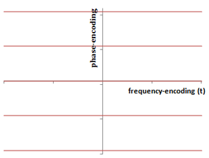
Illustration of the layout of the K-space matrix. The frequency-encoding direction is along the x-axis in K-space (may or may not be that axis in the image, if it is rotated); this represents the time samples of the signal. The y-axis is the phase-encoding direction: each phase-encoding step yields a separate horizontal line. The center of K-space contains the contrast, and the periphery contains the resolution. The spacing in K-space represents the field-of-view.

As we've alluded to in the sections above, the MR scanner samples and digitizes the signals it obtains from each phase-encoding run and stores the data in a matrix, which is known as K-space. The reason for the letter k is apparently 'lost in the mists of time' but just represents a mathematical convention when talking about Fourier transforms. It is worthwhile briefly discussing the appearance and properties of K-space, as understanding K-space is required to better understand reduced K-space acquisitions and non-Cartesian trajectories.

Matrix size. The number of points we need in the K-space matrix is known as the matrix size and often referred to as N. Usually, we describe the matrix size by its dimensions, e.g. 256 x 256. This means that we will need 256 samples of the signal and 256 phase-encoding steps. The Fourier transform (well, the digital, or discrete, Fourier transform) takes a matrix in K-space and returns a matrix of the exact same size in image space. That means that the matrix size determines our final image size (not field of view but size of the actual picture, in pixels). For a fixed field of view, increasing the matrix size gives greater resolution.

Frequency-Encoding direction. Traditionally, the x-axis of K-space is the frequency-encoding direction and represents the samples (measurements) of the echo in time. The echo is measured from -T/2 to +T/2 for a total time of T. The amount of time we need to sample, T, depends on the bandwidth of the frequency-encoding gradient. Simply put, the stronger the gradient, the larger the range of frequencies (since there will be a larger range of B) - and with a wider range of frequencies, the maximum frequency will be higher. That will necessitate faster sampling (again, twice as fast as f_max). We gain an advantage - since we only need N samples, the higher the sampling rate, the less total time it takes to get the samples.

For example, let's say we have a matrix size of 256. For a bandwidth of 2*16 = 32 kHz (i.e. maximum frequency is 16 kHz spanning -16 to +16 kHz), for the Nyquist limit, we need to sample at 32 kHz = 32,000 samples/s = one sample every .03 ms. Thus, the total sampling time is 256*.03 = 8 ms. If we decrease the bandwidth, then we can sample more slowly - although this takes longer (since there is more spacing between the samples). While that may seem like a disadvantage, it turns out that the longer we sample, the better the signal-to-noise. You can play with the effects of changing bandwidth on the MRI simulator in the section on image formation parameters.

Aliasing could occur in the frequency-encoding direction if we do not sample frequently enough - hence sampling at twice the maximum frequency as discussed above. However, the bandwidth represents the range of frequencies in the field of view. Any body parts outside the field of view will have a wider frequency variation (they're farther to the side and thus experience a stronger effect of the gradient). Thus, we have to take these into account as well in order to prevent unexpected aliasing - which will corrupt our image. The scanner will often sample at twice the necessary rate to prevent this.

Phase-Encoding direction. The y-axis of K-space typically represents the phase-encoding direction. No phase-encoding (gradient off) is plotted at the center, and increasing positive and negative strengths of the gradient are plotted above and below the center axis. As we mentioned, if the matrix size is 256 x 256, that would mean that we need 256 phase-encoding steps. What determines the number? As with the frequency encoding direction, the 'sampling rate' - or spacing between the phase-encoding steps - corresponds to the maximum range of phase shifts we can measure. Since phase shift is linearly related to position along that axis, the spacing of phase-encoding steps represents the field-of-view. The signal (echo) obtained after each phase-encoding step (and while the frequency-encoding gradient is on) is stored as a line of k-space. Once all of the lines are acquired, the matrix can be Fourier transformed to yield the image.

Aliasing is much more common in the phase-encoding direction. This is because each phase-encoding step takes an entire MR excitation step (i.e. 90 and 180- degree pulses followed by readout) and thus takes up a lot of time. In order to minimize the total time, we may skimp on phase-encoding steps (increasing their spacing to decrease the field of view). As we've mentioned, if you do not sample frequently enough - in this case, in the phase-encoding direction - you will get aliasing. This results in overlap of tissue outside the field-of-view onto the body part of interest. You can experiment with reduced K-space acquisition in the simulation to see how this works. Parallel imaging takes advantage of coil sensitivities to 'unwrap' the aliasing.

Signal in K-space. If you look at a plot of K-space (the amplitude of signal at each point), you will see a bright spot at the center and darkness around the periphery. This is a result of dephasing. The center represents time = 0 and no induced phase shifts. As you can see from the simulations in Frequency and Phase encoding, the more different frequencies and phases present in a signal, the smaller the total signal, especially over time (see the top right panels in the simulations, the gray line represents the total signal). This is just because the signals get out of sync with each other over time if their frequencies are different - and thus, the valleys and peaks start to cancel each other out. A phase shift makes the signals out of sync from the very beginning, making the 'cancellation' even more apparent. (In sound, one might refer to this process as destructive interference.)

Contrast and Resolution. As we've mentioned before, matrix size determines the eventual resolution of the image. Thus, cutting out the periphery of K-space, which reduces the matrix size, decreases resolution. As another way to think about it - the periphery of K-space contains resolution information. Again, the spacing of lines in K-space (sampling rate in time, or in phase encoding) represents field of view, which isn't changed by cutting out the periphery.

The contrast information - brightness of organs, large lesions, etc. - lies in the center of K-space. Why? In the phase-encoding direction, the center of K-space represents low or no phase-encoding - thus, there is no distinguishing different points along the phase-encoding direction. The signal obtained with poor resolution just represents the overall brightness of the larger structures in the image - thus, the contrast. Similarly for frequency encoding, without the high-resolution information in the periphery, the (much brighter) signal we have in the center of K-space represents the brightness of the large structures.

Understanding these points lets us manipulate K-space for faster imaging. We will not discuss these in any detail here but simply give some examples. We may wish to pursue a strategy of oversampling the center of K-space, where all the contrast is, if we want faster imaging and care much more about contrast than spatial resolution. This strategy is employed for time-resolved MR angiography by some vendors (e.g. TWIST by Siemens or TRICKS by GE). Alternatively, one may want to reduce motion artifact - which is caused by motion in between the phase-encoding steps. Using a radial pattern of K-space acquisition, instead of a rectangular pattern, motion artifacts can be reduced (e.g. BLADE or PROPELLER sequences).

References

1. Hashemi, R. H., Bradley, W. G. & Lisanti, C. J. MRI: the basics. (Lippincott Williams & Wilkins, 2010).
2. Mezrich, R. "A perspective on K-space." Radiology. 1995 May;195(2):297-315.
3. Carroll, TJ. "The Emergence of Time-Resolved Contrast-Enhanced MR Imaging for Intracranial Angiography." AJNR Am J Neuroradiol. 2002 Mar;23(3):346-8. PMID: 11900996.

---

Images and Content Copyright 2014 Mark Hammer. All rights reserved.