MRI Physics: Parallel Imaging in MRI

Introduction to Parallel Imaging | SENSE | SMASH | Go Home

This parallel MRI simulation will give you a sense of how parallel imaging (specifically, the SENSE algorithm) works. Play around with the number of coils and acceleration factor to see what happens. Note that the simulation is computationally intensive so there may be a bit of a delay as you change parameters. (Also, note that the coil sensitivities are positioned as bands across the patient instead of at the periphery, as it would be with real surface coils.)

Parallel Imaging Parameters:

Number of Coils:
2 4

Noise:
low high

Acceleration Factor:

2 3 4

SNR:

Introduction to Parallel Imaging

One of the major challenges in MR imaging is acquisition time. The major contribution to imaging time is the number of phase-encoding steps (PE), as

Time = N * PE * TR / ETL

There are several traditional ways of decreasing the number of phase encoding steps, which are detailed on the main MRI Image Formation Parameters page. One clever way of doing it, though, is to utilize parallel imaging. The initial impetus for this technique came as people shifted from using volume receiver coils to phased-array coils, which are composed of an array of surface coils that cover the whole volume. The advantage of using surface coils is that they're sensitive to a much smaller volume of space and thus can pick up signal from the body part without too much extra space, which only contributes noise. However, the adoption of phased-array coils also inspired the development parallel imaging.

Volume Coil Phased-Array Coil

Diagram of a volume coil (e.g. birdcage head coil) on the left and phased-array receiver coil on the right. The volume coil receves signal from the entire enclosed volume, while the separate coils (really, coil groups) in the phased-array send separate information back to the scanner computer. See that the amount of signal from each coil is different at every location.

As you can see, each surface coil within the array is sensitive to a different part of the volume. This leads to the idea of using the coils themselves to help localize MR signals. Now, recall that you can decrease the number of phase-encoding steps while keeping the same resolution by increasing the spacing between them; this results in a reduced field-of-view (see MRI Image Formation Parameters for a review). This works fine when the entire body part is covered in the smaller field of view; however, if there are parts outside of this field of view, they wrap into the region of interest and obscure anatomy. This phenomenon is referred to as aliasing (because it results from undersampling the signal, with resulting incorrect phase or frequency assignment by the Fourier transform.)

The idea of parallel imaging is to combine the spatial localization provided by individual coils (or coil groups) in a phased-array to "unwrap" the aliasing caused by a reduced field of view. Thus, by using a little bit of math, we can reconstruct the full field of view without actually acquiring those extra phase-encoding steps. The ratio of the reduced phase-encoding steps to the full set is referred to as the acceleration factor or R, and this represents the time-savings factor (and also the size of the decreased field of view).

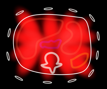
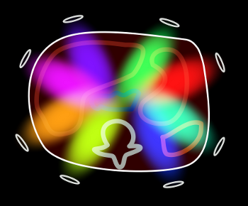
The first step in doing parallel imaging is to find out the spatial sensitivites of each coil (or coil group). This is typically done by acquiring a very low resolution image of the body part. The data from all coils are combined to form an average image (sometimes called sum of squares since that is one way of calculating it). By dividing each individual coil's image by the average, you get the sensitivity profile. You can see these steps in action in the simulation above.

SENSE

The simplest type of parallel imaging is called SENSE (Sensitivity Encoding), and this is what we will focus on here. SENSE involves using the spatial (real space as opposed to k-space) sensitivities of each coil to unwrap aliased images. The simulation above implements the SENSE algorithm, which is described and diagrammed below.

SENSE reconstruction

Spatial aliasing and the SENSE reconstruction (artistic rendition). Left, the body part lies in a phased-array of 2 coils, one anterior and the other posterior; the gradient shows that the anterior coil picks up much more signal from anterior tissues than posterior tissues. The dashed lines show the field of view when we do a reduced field-of-view acquisition. Right, the reduced field-of-view image. Notice the white circle in the aliased image (point P) is a superposition of two points in the body (voxels V1 and V2). The anterior coil receives different strengths of signals from the two points.

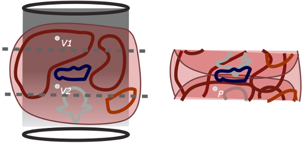
As you can see from the figure, SENSE takes advantage of the fact that we know the relative signal strengths from each coil at each point, and we know where each point in real space maps to on the aliased image. We have already found the coil sensitivities for each coil. We also have just acquired the aliased images, recording the signals from each coil separately. Then we can solve some simple equations. Let's let P be the white dot in the aliased image. This point actually represents two voxels in real space, V₁ and V₂ that are superimposed. Finally, let's call the coil sensitivities C_ant and C_post for the anterior and posterior coils. Then

Signal_{ant, P} = C_{ant, V1} * Signal_V1 + C_{ant, V2} * Signal_V2

Signal_{post, P} = C_{post, V1} * Signal_V1 + C_{post, V2} * Signal_V2

These are two equations for two unknowns (Signal_V1 and Signal_V2). This works the same for any number of coils and acceleration factor, as long as R ≤ coils.

As R increases, the amount of wrap increases - specifically, the number of voxels that wrap onto the same point is equal to R. Thus, as R gets larger, the reconstruction is more difficult. Since the number of voxels that wrap is equal to R, this explains why the number of coils you need must be at least as big as R in order to reconstruct the image. Basically, for each voxel you want to reconstruct, you need to have a coil with a unique sensitivity for that point in space. Realistically, depending on where the coils are located, you may need even more coils than that because some coils may not be able to discriminate between parts of the body that are far away.

Of course, parallel imaging comes at a cost - decreased SNR. Just like with traditional reduced field-of-view (and other techniques of reducing acquisition time), the less time you sample the body part, the worse your signal. The equation is pretty much the same as traditional reduced field-of-view but with an extra factor g related to coil geometry:

SNR = SNR_initial / (g * √R)

Because of the signal loss (and coil geometry), there is a limit to the acceleration factor you can use, which is usually up to 3-4.

SMASH

As noted above, SENSE reconstructs the image using spatial sensitivity to unwrap aliased images in real space. However, there are some disadvantages to this approach. In particular, actually finding the coil sensitivities - which has to be done for each patient - is problematic in regions where there is very low signal (the noise dominates). This is especially relevant in the chest, where the signal-poor lungs take up a large part of the field of view. The result of this is reconstruction artifacts, which can obscure the anatomy of interest. An alternative to SENSE is reconstruction in k-space. The simplest of these k-space approaches is called SMASH (which stands for Simultaneous Acquisition of Spatial Harmonics). The concept is exactly the same as for SENSE, but the mathematical reconstruction is done on the k-space images (and k-space coil sensitivities) rather than in real space.

Another problem with coil sensitivities is that they depend a lot on the position of the patient (or body part) in the scanner. In the traditional SENSE and SMASH approaches, the coil sensitivites are acquired before the full-resolution scan by a quick, low-resolution scan. If the patient moves - or breathes - between the two scans, it can completely mess up the reconstruction. One way to fix this would be to somehow acquire both the low resolution, full field of view scan and the high-resolution, reduced field of view (aliased) scan at the same time. This can actually be done by oversampling the center of k-space during the accelerated scan. In other words, one scan will acquire the central lines of k-space in the normal spacing but the peripheral lines spaced by R. The central lines are used to make the coil sensitivities, which are then used to reconstruct the full field-of-view image in the normal way. These techniques are known as mSENSE (spatial reconstruction) and GRAPPA (k-space reconstruction).

Things to remember:

Parallel imaging represents a way to speed up acqusition time by undersampling the phase-encoding direction by an acceleration factor R.
It requires the use of phased-array receiver coils to localize signal based on proximity to each coil in order to unwrap the aliasing caused by the undersampling.
When accelerating by a factor of R, the signal-to-noise drops (by 1/√R) as you are acquiring fewer samples. The highest R you can use is the number of independent coils you have, but often you cannot even go that high.
Traditional parallel imaging requires acquiring an initial, low-resolution image to determine the spatial sensitivities of each coil, but newer techniques acquire that information in the accelerated scan itself.

References

Hashemi, R. H., Bradley, W. G. & Lisanti, C. J. MRI: the basics. (Lippincott Williams & Wilkins, 2010).
Blaimer M, et al. "SMASH, SENSE, PILS, GRAPPA: how to choose the optimal method." Top Magn Reson Imaging. 2004 Aug;15(4):223-36. Pubmed.
Glockner, J. F., et al. "Parallel MR Imaging: A User’s Guide." Radiographics 2005 Sept; 25(5): 1279. Radiographics.