MRI Physics: Flow Related Effects in MRI

Flow Voids

The first flow-related phenomenon we'll discuss is the flow void. This only occurs in spin-echo (and fast spin echo) sequences, typically with T2 weighting. Fast moving blood experiences the 90-degree pulse but misses the 180-degree rephasing pulse, so its signal decays before the echo is read out.

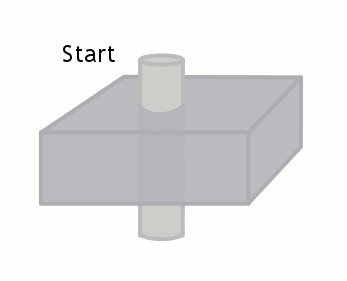
The time between the 90 and 180-degree RF pulses is TE/2, so if the blood flows through the slice (with thickness Δz) faster than TE/2, no signal will be obtained. As an equation, a signal void will be seen if, for blood velocity v,

v ≥ Δz / (TE/2)

Some things to remember:

• Some references refer to this flow void phenomenon - related to the 90 + 180 pulses - as a time of flight effect (not to be confused with TOF angiography).
• Flow voids from TOF effects only occur with spin echo (and fast spin echo) sequences, since gradient echo sequences do not have 180 degree RF pulses. You can get signal loss from flowing blood in gradient echo sequences because of flow-related dephasing - see below.
• Flow voids are more pronounced on T2-weighted sequences because those have longer TEs (i.e. longer times for the blood to move between the two pulses).
• We can take advantage of the same concept to generate the black-blood images in cardiac MRI. These exaggerate the flow void effect by employing an inversion pulse to null signal from moving blood, but a full discussion is beyond our scope here.

Flow-Related Enhancement

In many ways, this is the opposite of the flow void phenomenon. Flow-related enhancement is typically seen in gradient echo sequences (which do not have the 180-degree rephasing pulse and typically use very short TEs, making any flow void effect negligible). When an MR scanner images a slice of tissue, it subjects the tissue to multiple 90-degree pulses to flip the magnetization into the transverse plane and also cause T1 weighting. Remember that after the first 90 degree pulse, the tissue is only allowed to recover a certain fraction of its longitudinal magnetization - determined by TR - in order to give T1 weighting to the image. The longer the TR, the more recovery occurs, and the less T1 weighting.

Of course, this only happens if the tissue stays put and is subjected to these multiple pulses. If fresh blood flows into the slice, it will start out with all of its longitudinal magnetization. Therefore, after a 90-degree pulse, it will have a lot more transverse magnetization than the surrounding tissues. This will make it bright on the images (seeming like it has a short T1).

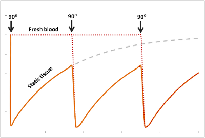
The degree to which this effect occurs depends on the velocity of the blood and the TR of the sequence. It also depends on the direction of scanning - if the scanner has already saturated the blood entering the slice because it came from the slice just before, then this effect will be less or nonexistant.

In order for new blood to replace old blood in the slice, it has to come in after one 90 degree pulse and before the next one, i.e. it must flow through the slice faster than TR. If it is slower than TR, it will get hit with a 90 degree pulse at some point during the imaging. So for blood velocity v, flow-related enhancement will occur if:

v ≥ Δz / TR

A couple of points to remember:

• Note that flow-related enhancement occurs at much lower velocities than required for the time-of-flight flow voids - this is because it depends on TR instead of TE (and TR >> TE for most sequences).
• This effect is particularly strong in gradient echo sequences, which do not have time-of-flight effects and tend to have short TRs. The short TEs of gradient echo sequences minimize flow-related dephasing, as well.
• Flow-related enhancement depends on the slice orientation and the direction of scanning (i.e. cranial-caudal or vice versa) compared to the direction of the blood flow itself. If the protons in an adjacent slice have been saturated before flowing into the current slice, flow-related enhancement will be diminished or nonexistant; if blood is flowing within a slice, there will be no enhancement.
• This same concept can be harnessed for time-of-flight MRA. If you entirely saturate the protons in a slice, then the only protons with signal will be blood flowing into the slice.

Phase Shifts

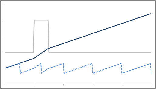
Let's first review how radiofrequency (magnetic field) gradients cause phase shifts in precessing protons. (For more details about how gradients are used for phase encoding, see the section on Spatial Localization.) Remember that when a magnetic field gradient is on, the protons precess with a slightly different frequency since they experience a magnetic field slightly greater or lesser than B₀ (the amount depends on their position and gradient strength).

After the gradient is turned off, they revert to the same frequency as all the other protons, precessing in the uniform magnetic field of the magnet. But, they 'remember' their experience in the gradient by keeping a phase shift. In other words, they rotate 'off cycle' from the other protons. The picture below illustrates this point.

Mathematically, we can look at it like this: The signal we measure - transverse magnetization - depends on the angle of the precessing proton. This angle changes over time in a constant motion depending on the Larmor frequency (designated here by ω): angle = ω * t . We can describe a phase shift by just imagining that we bump up the angle by a certain constant (designated here by φ), so that

angle = ω * t + φ

Now, let's say that we speed up the frequency for a short while to F₁, so

angle = F₁ * t + φ

And now we turn off the gradient after some time T₁. The angle now measures F₁ * T₁ + φ. As the proton continues to precess at its native frequency ω, its angle then measures

angle = ω * t + F₁ * T₁ + φ

As you can see, the angle remembers each of its phase shifts. Of course, angles can only measure up to 360 degrees - after that, it wraps around from 0 again.

Flow-Related Dephasing

Protons that are moving (e.g. in blood) experience different magnetic field strengths, as gradients vary in space. While they will precess at the same frequency as the stationary protons around them when they're in the slice, they will still 'remember' the phase shifts from those earlier different frequencies. This phenomenon is called flow-related dephasing.

You can see that moving protons accumulate an additional phase shift when compared to stationary protons. However, flow-related dephasing is actually helpful sometimes:

• We can take advantage of this phenomenon to measure velocity of moving blood - this is called Phase-Contrast MR Angiography.
• This dephasing will show us areas of turbulent blood flow, such as stenosis or regurgitant gets from dysfunctional heart valves.

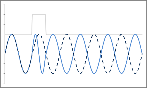
But let's say we want to neutralize these effects (actually, we need to do this to properly calibrate both phase-contrast MRA and bright-blood cardiac MRI). We need to change our gradients so that they 'balance out' - and protons moving with constant speed end up without a phase shift. Let's first try a biphasic gradient - half of the time it will give a positive phase shift, while the other half of the time it will give a negative phase shift:

The stationary protons end up with no net phase shift at the end, but the moving protons do have a phase shift. Why is that? Well, as you can see, the gradient is stronger as the proton moves farther out - therefore, while the amount of time is balanced, the second half of the gradient pulse actually causes a greater phase shift. This biphasic gradient is exactly what we want for Phase-Contrast MR Angiography; if we measure the phase shift, we know how far - and therefore how fast - the proton was moving.

In order to fully compensate for moving protons, we need to add another phase (or "lobe") to the gradient pulse. Remember that the gradient is stronger as the proton moves out, so we need an extra 'kick' at the end. The gradient also has to balance out overall so that stationary protons do not end up with a phase shift. We can use a triphasic gradient, as you see below; the ratio of the lobes is 1:-2:1 (which adds up to 0).

In this example, the phase shift of both moving and stationary protons is zero at the end. Thus, moving protons will end up with the same amount of signal as stationary protons. This is what is done to create a control image for phase-contrast MRA (for background subtraction). It's also what happens in bright-blood cardiac MRI sequences, so that you can see the blood without all sorts of dephasing artifacts as it moves through the heart.

Now, one thing we haven't focused on is the dynamics of the proton motion. It turns out that the triphasic gradient only works if the proton moves at a constant speed. If it's accelerating or decelerating - things that often happen in stenotic jets, for example - then you will get dephasing. You can add extra lobes to the flow-compensation gradient (e.g. 5 lobes instead of 3), but the more lobes you add the longer it takes to make the gradient.

Some things to remember:

• Flow-related dephasing is greater in sequences with longer TEs (this exaggerates the dephasing, as there is a longer delay before the echo is measured).
• The simplest flow-compensation gradient has 3 lobes, but this will only work for protons moving at a constant speed.
• The more lobes you add, the longer it takes - so your minimum TE increases. That leads to lower signal because of T2 (or T2*) decay.
• Turbulent flow, as happens with stenotic jets for example, is so 'random' that flow compensation cannot ever fully compensate.

Pulsation Artifacts

Most of the artifacts discussed above relate to essentially constant blood flow. However, as we all know, arterial blood does not move constantly; rather, velocity dramatically increases in systole and decreases during diastole. This phenomenon is responsible for the patient's pulse, obviously, and produces artifacts in the MR image as well. Recall that in MR imaging, the phase encoding process takes place over a relatively long period of time (up to several seconds). This timeframe is long enough for physiologic processes to occur within the imaging slice, including cardiac and respiratory motion. Since some lines of k-space are acquired while the body is in one state (e.g. systole) and others while the body is in another state (e.g. diastole), this introduces an artifact in the MR image. The artifacts produced by bulk respiratory or cardiac motion are directly discussed in the page on MRI artifacts.

As discussed in the above sections, moving protons accumulate a phase shift because they experience slightly different gradient strengths than adjacent stationary tissue. If this flow were constant throughout the imaging process, you would simply see flow-related dephasing and perhaps some pixel misregistration (recall that phase is used to determine proton localization). However, pulsatile flow means that during some portion of the imaging process, the blood in the vessel is relatively stationary or slow moving, while at other times it is fast-moving. Thus, the phase shift within these vessels will be different during different parts of the cardiac cycle. Of course, the scanner and Fourier transform assume that the imaging slice does not change during the course of imaging - so these changes produce artifacts. These artifacts, often referred to as ghosts since they are faint images of the original vessel, are seen along the phase encoding direction since some phase encoding steps will occur during systole and others during diastole. (Frequency encoding takes place over milliseconds and so is much faster than the cardiac cycle.)

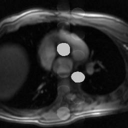
Simulation of pulsation artifact (vascular ghosting), with phase encoding in the AP direction.

It is important to realize that the direction of the artifacts is independent of the direction of blood flow. The phase shift accumulated by the protons will depend on their velocity and direction of flow, but the artifact is always seen in the phase encoding direction because it results from changing phase shifts during the phase encoding process. For example, even in cases of blood flowing out-of-plane, such as the simulated image above, the ghosts are produced in-plane, in the phase encoding direction. Because the heart rate is constant, it produces regularly spaced ghosts in the phase encoding direction. (Advanced mathematics note: If the pulsatile process were a simple sine wave, there would only be a single image produced, with a shift related to the frequency of the pulse. However, blood flow pulsatility has a more complex shape, as it tends to peak quickly and fall of slowly, so this produces multiple images corresponding to multiple frequency components in the pulse waveform.)

Vascular ghosts can occasionally simulate pathology (famously, the aorta can simulate a segment 4 liver lesion). If the ghosts obscure important anatomy, one can switch the phase encoding direction, which will change the direction of the artifact. Using flow compensation gradients or black blood imaging will reduce this artifact, as well.

References

1. Hashemi, R. H., Bradley, W. G. & Lisanti, C. J. MRI: the basics. (Lippincott Williams & Wilkins, 2010).

Copyright 2013 Mark Hammer. All rights reserved.