CT Physics: CT Reconstruction and Helical CT

Back-Projection | Helical CT and Pitch | Go Home

This CT simulation illustrates the technique of CT reconstruction. Change the fan beam angle and see how that affects the field of view. Backprojection ("raw backprojection") and filtered backprojection reconstructions are displayed.

Image: Fan Beam Angle:

Explanation of Backprojection

In order to understand CT reconstruction, we first need to understand how the computed tomography scanner works. Really, it is quite simple: it simply takes images of the body part at multiple angles (or projections) around the body. You can see what any given projection looks like in the simulator above. For any given angle, the projection is a line of brighter and darker pixels depending on how much attenuation blocks that part of the beam. Sometimes people talk about sinograms, which are simply a display of all of the different projections for a given slice stacked together. The sinogram has (sinusoidal) undulations as the CT tube rotates around the patient, which is how this image got its name.

Backprojection. The standard method of reconstructing CT slices is backprojection. This involves "smearing back" the projection across the image at the angle it was acquired. By smearing back all of the projections, you reconstruct an image. This image looks similar to the real picture but is blurry - we smeared bright pixels across the entire image instead of putting them exactly where they belonged. You can see this effect in the simulator on the right-most panel.

In order to reconstruct an image, you need 180 degrees of data (* actually 180 + fan beam angle). Why? The remaining 180 degrees are simply a mirror image of the first (because it does not matter which way a photon travels through tissue, it will be attenuated the same amount). (Because of the fan beam geometry, you need to measure an extra amount - equal to the fan angle - to actually get all of the data you need, but the concept is the same.)

In a fan-beam geometry, the angle of the fan determines how much of the object is included in the reconstructible field of view. A point must be included in all 180 degrees of projections in order to be reconstructed correctly.

Filtered Backprojection. As you may have noticed, backprojection smears or blurs the final image. In order to fix the blurring problem created by standard backprojection, we use filtered backprojection. Filtering refers to altering the projection data before we do the back-projections. The particular type of filter needed is a high-pass filter, or a sharpening filter. This type of filter picks up sharp edges within the projection (and thus, in the underlying slice) and tends to ignore flat areas. Because the highpass filter actually creates negative pixels at the edges, it subtracts out the extra smearing caused by backprojection. Thus, you end up with the correct reconstruction (see the simulator panel labeled "Filtered BP Reconstruction").

Left: Unfiltered back-projection. Right: Filtered Back-projection.

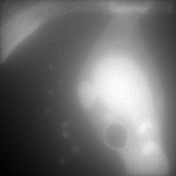
Where's the catch? Well, real CT data contains noise. Unfortunately, the high-pass or sharpening filter accentuates this noise (because noise looks like jagged edges). Thus, if we were to use a simple high-pass filter our CT images would look too grainy. In order to get around this, we use filters that are slightly 'softer' than a simple high-pass filter. How soft the filter is (i.e. how much noise does it throw out) is referred to as the 'reconstruction kernel'. We choose different kernels based on what type of image we are trying to create. For imaging the lungs or bones, we are looking for small, discrete features (i.e. fractures, nodules, fine reticulation). Thus, we want to use a hard (sharp) kernel to accentuate these features. For soft tissues such as the brain or abdomen,we are looking for larger features with mild differences in attenuation (e.g. liver lesion). Thus, for these tissues, we prefer a softer kernel that will decrease noise. Of course, these images are also viewed at different window settings because of the underlying attenuation values of these tissues. In fact, the two phenomena are somewhat related - we can use noisier kernels in situations where the inherent contrast is very high, e.g. lung vs air or bone vs soft tissue. The high contrast means that there is a big difference in attenuation, much bigger than the noise. We have to use softer kernels where there is less contrast and we really need to remove noise.

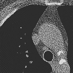
Left: Soft kernel smoothes the image. Right: Sharp kernel shows edges better but with more noise.

One important thing to realize is that the edge enhancement of sharp kernels can create artificially high attenuation at sharp edges. In particular, some small lung nodules may appear calcified on sharp kernel images, when they are truly not. (You may notice that small blood vessels will appear similarly dense.) It is important to measure attenuation only on soft kernel images.

Iterative Reconstruction. You may wonder if there is a better way to solve the noise problem. In fact, there are other reconstruction techniques than backprojection, and the most common of these is iterative reconstruction. These algorithms are much more computationally intensive than backprojection since they aim to account for noise and other artifacts. The iterative nature of the algorithm means that it takes an initial guess and refines it over several tries. Iterative reconstruction typically starts with a regular filtered backprojection image. It then simulates making a CT reconstruction of this initial guess. By looking at the difference (or 'error') in the reconstruction, you can make a better guess. This process then repeats for a defined number of cycles.

The simulation used by iterative reconstruction techniques attempts to model real-world noise and attenuation processes. Thus, it tends to perform better in high-noise situations (e.g. low radiation dose scans) and in situations with very high attenuation (e.g. metal implants). As noted, the trade-off tends to be much longer reconstruction time; the images also have a different subjective quality than filtered backprojection.

Helical CT and Pitch

Image: Pitch: Radiation Dose: %

Helical CT. Early CT scanners imaged one slice of the body at a time before moving to the next slice. Thus, the thickness of the slice depended only on the thickness of the CT detector. Because scanners collimate the beam to the width of the detectors, slice thickness can also be said to equal the collimator width.

Current CT technology makes use of a so-called helical (or "spiral") path. In helical CT, the scanner is constantly spinning and the patient table is constantly moving. Thus, no two CT projections are acquired at the same slice (z-position) in the body. If the table is constantly moving, what then constitutes a slice that the scanner will reconstruct? Modern helical CT averages (or 'interpolates') data from two projections 180 degrees apart. A photon will see the same attenuation whether it passes through tissue 'forward' or 'backward' - so that angles 180 degrees apart are equivalent. This interpolation is done to convert the helical path to transverse slices (see what happens in the simulation if you only reconstruct 180 degrees - you get spirals). This also explains the concept of slice broadening - each point reflects data from two z positions, separated by how far the table moves as the beam turns 180 degrees. As before, the thickness of tissue included in a single projection is the collimator width (often 0.7-1 mm).

The relationship between speed of rotation and speed of table movement is referred to as pitch. In particular,

Pitch = Table movement in 360 degrees / Collimator width

If Pitch = 1, then the next 360 degree circuit starts adjacent to where the last one started, with no gap. If pitch < 1, then there is overlap among the helices. If pitch > 1, then there are gaps in the helix (but not the reconstruction). Generally pitch is kept between 1 and 2. At a pitch of 2, 180 degrees of rotation brings the table a distance of one collimator width. If pitch > 2, then there are gaps in the reconstruction. (Remember, each projection uses data from 2 projections spaced by 180 degrees.)

Pitch:

Illustration of the helical CT scan. The helical path of the beam is drawn in blue. A single 360-degree rotation of the tube is shaded in red. Slices in helical CT are reconstructed by using interpolated data from two projections 180 degrees apart; this causes slice broadening, where the amount of tissue included is slightly greater than the collimator width. An example tissue slice (from two projections 180 degrees apart) is highlighted in green.

The advantage of helical CT is that it is much faster than the step-and-shoot procedure since the entire scan is acquired in one fluid motion. Increasing pitch increases the speed of the scan. However, this comes at a disadvantage as information in the gaps between helices is lost; this causes reconstruction artifacts and can obscure small features like nondisplaced fractures or small lesions (see simulation above). Decreasing pitch improves image quality but increases the radiation dose to the patient as more positions are being radiated. For more discussion on how pitch affects patient dose, see the section on dose in CT.

Multidetector row CT. Multidetector row (or multi-slice) CT uses multiple rows of CT detectors instead of only one. (Even single-detector row CT has multiple detectors along the gantry, but it has only one row, i.e. it only obtains a single slice along the z direction.) The advantage of MDCT is faster scanning, as more of the body is contained in each turn of the gantry. For MDCT, multiple slices are reconstructed per projection by the multiple rows of detectors. In MDCT, pitch is calculated by dividing the table movement by the entire beam width. This yields numbers similar to the one-slice version: a pitch of 1 corresponds to contiguous helices. To read more about MDCT, see the section on cardiac CT.

Slice thickness and Reconstruction interval. In step-and-shoot CT, slice thickness and slice spacing are the same - each time you scan one slice, you move to the next slice and start again. However, in helical CT, you are continuously scanning the entire patient. This decouples the selection of slice thickness from slice spacing (reconstruction interval). With single-slice CT, the slice thickness is determined by the detector width - with mild slice broadening just based on the pitch of the helical scan. With MDCT, slices can be composed of a single detector thickness or multiple adjacent detectors. For example, if you have 2.5 mm detectors, you can either create 2.5 mm slices (well, slightly broadened by helical technique), or you can create 5 mm slices by adding the data for two adjacent detectors.

Reconstruction interval - the spacing between adjacent slices - is independent of slice thickness in helical CT. The z-position of any given slice is determined by which projection is used to start the slice. Remember that to reconstruct an entire slice, you need 180 (plus fan angle) degrees of projection data. In helical CT, each projection is done at a different z-position - therefore, depending on which projection you use to start the slice, your slice is centered at a different z-position.

Slice Thickness:	3 mm
Reconstruction Interval:

Illustration of helical CT reconstruction of successive slices. Depending on the reconstruction interval, slices may overlap. In that case, at any given time, data may be acquired for multiple slices. An entire slice is completed when the gantry has covered 180+fan angle degrees.

The reconstruction interval is thus determined by the software from the raw data the scanner obtained. You can reconstruct at any arbitrary interval - less than the slice thickness or even less than the collimator width. The slices remain the same thickness - but their spacing changes. Decreasing the reconstruction interval can have two advantages: (1) Increasing visibility of small lesions that may be obscured by volume averaging; if the lesion is centered in the slice, there is less normal tissue to average it out. (2) Improving stair-step artifacts in multiplanar reformats (MPRs); the multiplanar software will use the overlapping data to smooth out the MPR.

Things to remember:

Filtered backprojection is the standard method of CT reconstruction. Changing the filter yields a trade-off between noise and sharpness of the image.
Helical CT is much faster than step-and-shoot and is the standard method used in CT in the modern era.
Pitch is inversely related to radiation dose. CTDI_vol = CTDI_w / pitch. Increasing pitch decreases dose and speeds up the scan at the cost of slice blurring.
For most applications, pitch is kept between 1 and 2. This is not the case for cardiac CT and possibly some MSK applications.
In helical CT, slice thickness and reconstruction interval are independent. Slice thickness is determined by the detector width and pitch, while reconstruction interval can be chosen arbitrarily. The narrower the reconstruction interval, the better 3-D reconstructions.

References

Brink, JA, et al. "Helical CT: principles and technical considerations." Radiographics 1994 14(4):887.
Peters, T. "CT Image Reconstruction." Talk from 44th Annual AAPM meeting.